Graphs

A graph is made up of a set of vertices and edges that form connections between vertices. If the edges are directed, the graph is sometimes called a digraph. Graphs can be used to model data where we are interested in connections and relationships between data.

Definitions

• adjacent - Given two nodes A and B. B is adjacent to A if there is a connection from A to B. In a digraph if B is adjacent to A, it doesn't mean that A is automatically adjacent to B.

• edge weight/edge cost - a value associated with a connection between two nodes

• path - a ordered sequence of vertices where a connection must exist between consecutive pairs in the sequence.

• simplepath - every vertex in path is distinct

• pathlength number of edges in a path

• cycle - a path where the starting and ending node is the same

• strongly connected - If there exists some path from every vertex to every other vertex, the graph is strongly connected.

• weakly connect - if we take away the direction of the edges and there exists a path from every node to every other node, the digraph is weakly connected.

Representation

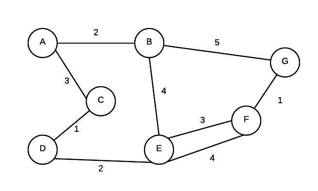
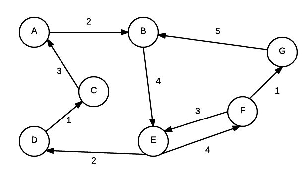
To store the info about a graph, there are two general approaches. We will use the following digraph in for examples in each of the following sections.

Adjacency Matrix

An adjacency matrix is in essence a 2 dimensional array. Each index value represents a node. When given 2 nodes, you can find out whether or not they are connected by simply checking if the value in corresponding array element is 0 or not. For graphs without weights, 1 represents a connection. 0 represents a non-connection.

When a graph is dense, the graph adjancey matrix is a good represenation if the graph is dense. It is not good if the graph is sparse as many of the values in the array will be 0.

An adjacency matrix representation can provide an O(1) run time response to the question of whether two given vertices are connected (just look up in table)

	A-0	B-1	C-2	D-3	E-4	F-5	G-6
A-0	0	2	0	0	0	0	0
B-1	0	0	0	0	4	0	0
C-2	3	0	0	0	0	0	0
D-3	0	0	1	0	0	0	0
E-4	0	0	0	2	0	4	0
F-5	0	0	0	0	3	0	1
G-6	0	5	0	0	0	0	0

Adjacency List

An adjacency list uses an array of linked lists to represent a graph Each element represents a vertex. For each vertex it is connected to, a node is added to it's linked list. For graphs with weights each node also stores the weight of the connection to the node. Adjacency lists are much better if the graph is sparse. It takes longer to answer the question of two given vertices are connected (Must go through list to check each node) but it can better answer the question given a single vertex, which vertices are directly reachable from that vertex.

Dijkstra's Algorithm

Dijkstra's Algorithm is an algorithm for finding the shortest path from one vertex to every other vertex. This algorithm is an example of a greedy algorithm. Greedy algorithms are algorithms that find a solution by picking the best solution encountered thus far and expand on the solution. Dijkstra's Algorithm was first conceived by Edsger W. Dijkstra.

The general algorithm can be described as follows:

1. Start at the chosen vertex (we'll call it v1)

2. Store the cost to travel to each vertex that can be reached directly from v1.

3. Next look at the vertex that is least costly to reach from v1 (we'll call this vertex v2 for this examples

4. For each vertex that is reachable from v2, find the total cost to that vertex starting from v1 (we want the total cost, not just the lowest cost from v2). Update the cost of travel to these vertices if it is lower than the current known cost.

5. Pick the next lowest cost and continue.

Example

Consider the following graph (non-directed)

Graph for Dijkstra's shortest path example

Initial state

We will use Dijkstra's algorithm to find the shortest distance from A to every other vertex To track how we are doing, we will create a table that will track the shortest distance from A we have encountered so far as well as the "previous" node in the path (so if we follow all previous nodes, we end up back at A). We also track whether we "know" about the node... that is, have we already considered all paths starting from that node. Currently we do not know what nodes are reachable from A so we store infinity into every spot other than A. The cost of getting to A from A is 0. Initially the table looks like this:

Vertex	Shortest Distance from A	Previous Vertex	Known
A	0		false
B	$\infty$		false
C	$\infty$		false
D	$\infty$		false
E	$\infty$		false

Expand A

Now, starting from A, there are two vertices that reachable, B and E

We store the total distance from A into the table for both these vertices if it is less than the shortest distance so far. At this point, A is now known as we have considered all its neighbours

Vertex	Shortest Distance from A	Previous Vertex	Known
A	0		true
B	$\textbf{7}$	A	false
C	$\infty$		false
D	$\infty$		false
E	$\textbf{3}$	A	false

Expand E

Now, we continue from here by considering the unknown vertex that has the shortest distance to A. In this case it is 3 (smallest in distance table with a false value in known). In implementation, we actually would use a priority queue (heap) to store the vertex with its distance and simply dequeue the smallest distance and check that the vertex was still unknown.

In any case, we are going to now consider E. From E the unknown neighbours are B and D. The distance to D (from A) is 5 (3 + 2). The distance to B is 4 (3 + 1). Now, The value stored previously for D was $\infty$ so we replace that with 5. The distance to B was 7, so we replace that also. We also mark that E is now known

Vertex	Shortest Distance from A	Previous Vertex	Known
A	0		true
B	$\textbf{4}$	E	false
C	$\infty$		false
D	$\textbf{5}$	E	false
E	$3$	A	true

Expand B

The next vertex we consider is the one with the shortest distance to A that is still not known. This is now B.

From B, we can reach unknown neighbours C and D. The distance to C (from A) is 10 (4+6). The distance to D (from A) is 6 (4 + 2). The value stored in the table for C was $\infty$ so we replace that. The value stored in D was 5, so that entry is not replaced because this new distance is NOT smaller.

Vertex	Shortest Distance from A	Previous Vertex	Known
A	0		true
B	$4$	E	true
C	$\textbf{10}$	B	false
D	$5$	E	false
E	$3$	A	true

Expand D

The next vertex that with the smallest distance to A that is unknown is D. From D, there is only one unknown vertex (C). The distance to C is 9 (5 + 4). As this is smaller than what is stored, we will update the table

Vertex	Shortest Distance from A	Previous Vertex	Known
A	0		true
B	$4$	E	true
C	$\textbf{10}$	D	false
D	$5$	E	true
E	$3$	A	true

Expand C

The only vertex left is C. From C, there are no unknown neighbours so we mark C as known and we are done.

Vertex	Shortest Distance from A	Previous Vertex	Known
A	0		true
B	$4$	E	true
C	$9$	D	true
D	$5$	E	true
E	$3$	A	true

Shortest path

To find the shortest distance to A, we simply need to look it up in the final table.

However, if we want to find the shortest path it isn't so simple as a look up. We actually need to work away backwards by looking up the previous vertices. For example, to find shortest path from C, its previous was D. D's previous was E. E's previous was A. Thus, the path is:

A --> E --> D --> C